Theoretische achtergrond RFEM - Eindige Elementen
2 Finite Elements
2.1 Finite Elements from Topological Point of View
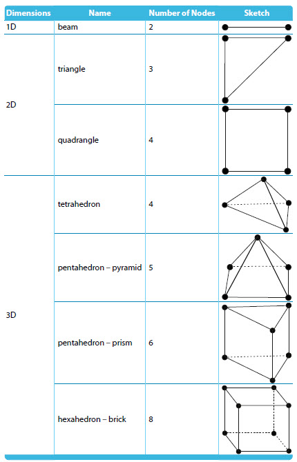
Table 2.1: Construction Models in RFEM
2.2 List of All Elements
The finite element types used in RFEM are given in the following table. They are chosen automatically by the program according to the situation.
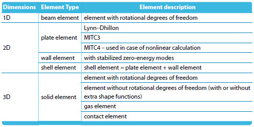
Table 2.2: Element description
2.3 Integration Procedure
For members, analytical integration is used for linear cases, while in the nonlinear setting the two point Gauss quadrature is used along the beam. For nonlinear cases the following integration rule is used in the cross-section: 2×2 Gauss quadrature for quadrangles and 4-point selective reduced integration rule for triangles (3 points for epsilon_x, epsilon_y and 1 point for gamma_xy).
In plate elements, analytical integration is used whenever possible (in Lynn–Dhillon element or in a triangular element). In other cases, a 2×2 composite Gauss quadrature is used in the element plane (quadrangles). In solids, a 2×2×2 composite Gauss quadrature is used in hexahedrons. Reduced one point integration is used for some particular terms to avoid numerical problems.
Let us focus on integration in plates with respect to their thickness, which is based on the Gauss–Lobatto quadrature. The Gauss–Lobatto quadrature is a Gauss quadrature in which boundary points are forced to also be integration points, which allows an exact evaluation of stresses on layer interfaces in case of multilayered plates. In case of linear calculation, three integration points are used per layer. In nonlinear calculation, nine integration points are used in the plate (nonlinear calculation allows one layer only).
2.4 Mesh Settings
Two mesh options exist in general:
- mapped meshing (= structural meshes)
- unmapped meshing
In the mesh settings, the user can define the element size, preference of the mapped meshing, and additionally has the possibility to generate only triangles or only quadrangles in surface meshes. Mapped meshes should be preferred due to better accuracy of stress results. In solid analysis for example, tetrahedrons give less accurate stress results comparing to analysis made on hexahedrons.
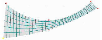
Figure 2.1: Mapped finite element mesh
2.5 Preventing Zero-Energy Modes
The following elements in RFEM can theoretically exhibit zero-energy modes: 3-node and 4-node quadratic wall elements, and all solid (4-, 5-, 6-, 8-) node elements with rotational degrees of freedom. In RFEM the so-called penalty stiffness is added. The stiffness is so small as not to influence results, but sufficiently high to prevent zero-energy modes.
2.6 Conforming Versus Non-conforming Elements
Non-conforming elements are those whose deformations and rotations are not continuous between elements:
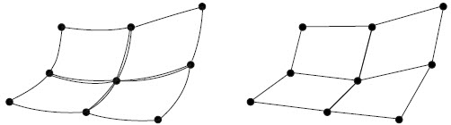
Figure 2.2: Left: non-conforming finite element, right: conforming finite element
The only non-conforming elements in RFEM are solid elements, which contain extra shape functions (ESF), i.e., linear solid elements without rotational degrees of freedom and linear wall elements.
2.7 Beam Finite Element
Beam (= member) finite elements contain displacement as well as rotational degrees of freedom.
2.8 Surface Finite Element
For bending components (i.e. for model plate and for bending components in a shell model) the following three finite element types are used:
- Chirkov element (Kirchhoff plates, linear or Picard calculation)
- Lynn–Dhillon element (Reissner–Mindlin plates, linear or Picard calculation, used up to RFEM 12.02.138917)
- MITC3 element (replacing the Lynn–Dhillon element from RFEM 13.01.140108)
- MITC4 element (Kirchhoff and Reissner–Mindlin plates, the Newton–Raphson calculation)
For membrane components (i.e. for model wall and for membrane components in model shell) the wall element is used. In shells, both elements for bending and membrane components are combined.
2.8.1 Chirkov Plate Element
The Chirkov element is a planar four-node element composed of four triangle elements used in case of Kirchhoff plates and linear calculation or nonlinear calculation based on the Picard method. The mid-element node is eliminated. The element uses the mixed formulation. Its unknowns are three displacements and three rotations in each node. For linear calculations, the Chirkov element is more precise than the MITC4 element. However, the eliminated node, which cannot be loaded by any force (it is eliminated under assumption of no loading), brings instability when it is used together with the geometric or material nonlinearity, where the Newton–Raphson method or other nonlinear iterative method is used. In this case the MITC4 element is used.
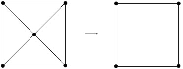
Figure 2.3: Middle node elimination.
For this element, the analytical integration method is used, therefore no zero-energy modes exist. Shear locking cannot occur in Kirchhoff plates.
2.8.2 Lynn–Dhillon Plate Element
The Lynn–Dhillon element is also a planar four-node element, composed of four triangle elements used in case of Mindlin plates and linear calculation or nonlinear calculation based on the Picard method. The mid-element node is eliminated. For linear calculations the Lynn–Dhillon element is more precise than the MITC4 element. However, the eliminated node, which cannot be loaded by any force (it is eliminated under assumption of no loading), brings instability when it is used together with geometric or material nonlinearity, where the Newton–Raphson method or other nonlinear iterative method is used. In this case the MITC4 element is used.
Figure 2.4: Middle node elimination.
For this element, the analytical integration method is used. Therefore no zero energy modes exist. Shear locking can occur in case of very thin plates, for this case the bound for shear stiffness is applied to avoid this problem.
2.8.3 MITC3 Plate Element
The MITC3 is an isotropic triangular element exploiting the mixed interpolation of tensorial components for the transverse shear terms to avoid shear locking, hence it is a more robust finite element, than the Lynn-Dhillon one. The price to pay is the lower order of approximation (linear, instead of quadratic), therefore a finer mesh is needed to achieve the same precision of results. It exploits the full 3-point Gauss integration for the stiffness matrix on the elements. In case of quadrangles, the aforementioned middle-node elimination technique is used for four triangles. Since RFEM 13.01.140108, MITC3 fully replaces the Lynn–Dhillon element, namely in linear static analysis, linear stability analysis, linear dynamic analysis, and nonlinear static analysis in case of first and second order theory without material nonlinearity and foundation.
2.8.4 MITC4 Plate Element
The MITC4 element is an isoparametric planar four-node element. A less precise element compared to the Lynn–Dhyllon element, but more robust in case of nonlinearities. The element uses linear base functions. For this element the full Gauss quadrature is used (2×2 integration points), which yields no zero-energy modes. Elimination of shear locking at decreasing thickness is done by the mixed interpolation of deflection, rotation and slope.
Figure 2.5: MITC4 element.
2.8.5 Wall Element
The element contains two displacements and one rotation per vertex. For walls and shells, the quadratic polynomial element with rotational degrees of freedom is used. This element is derived from eight-node/ six-node quadratic isoparametric element by mid-side nodes elimination. This element can theoretically suffer from zero-energy modes. In RFEM the so-called penalty stiffness is added. The stiffness is small enough not to influence results, but sufficiently big to prevent zero-energy modes. We can call this element quadratic, because it is based and derived from the genuine quadratic element, however, some additional simplifications are introduced so that the quadratic polynomial within the element is reduced. As a result, this element is more precise than linear isoparametric bricks, but less precise than genuine quadratic isoparametric bricks. On the other hand, computationally it is much more efficient contrary to the genuine quadratic element, because it contains no mid-nodes. If rotational degrees of freedom are not considered, a linear element with extra shape functions is used. The extra shape functions are used to avoid shear locking effects.
2.9 Solid Finite Element
All elements have three displacements and three rotations defined in each node, i.e., six unknowns per node. If setting Ignore rotational degrees of freedom in the Global Calculation Parameters dialog, then rotational degrees of freedom are not supported, all elements have only three unknowns per node. From all the elements listed above, hexahedrons are the most accurate and should therefore be preferred, if the construction allows the use of a mapped mesh. Especially tetrahedrons can offer less accurate results for stresses.
All solid elements which have both displacement and rotational degrees of freedom, can theoretically suffer from zero-energy modes. In RFEM, the so-called penalty stiffness is added. The stiffness is small enough not to influence results, but sufficiently big to prevent zero-energy modes.
Let us describe in more detail the hexahedron / brick elements. In RFEM the following two types are used (note that 4-, 5- and 6-node elements are analogously divided into the same two categories):
- hybrid brick elements with rotational degrees of freedom, used for the shell model
- linear isoparametric brick elements, used for the membrane model (with or without extra shape functions, also called bubble functions)
2.9.1 Quadratic Solid Element with Rotational Degrees of Freedom
Let us describe this kind of element on hexahedron. Hexahedrons have eight nodes, in each of which six independent components are defined (three displacements and three rotations), hence the element has altogether 48 unknowns. It is derived from the isoparametric quadratic element, which has nodes not only in vertices but also in the mid-sides. We can call this element quadratic, because it is based and derived from the genuine quadratic element, however some additional simplifications are introduced, so the quadratic polynomial within the element is reduced. As a result, this element is more precise then linear isoparametric bricks, but less precise then genuine quadratic isoparametric bricks. On the other hand, computationally it is much more efficient contrary to the genuine quadratic element, because it contains no mid-nodes.
2.9.2 Linear Solid Element with or Without Extra Shape Functions
Let us focus on hexahedrons. Hexahedrons have eight nodes, in each of which three unknown displacements are defined (no rotational degrees of freedom). The base functions are linear. From a theoretical point of view, it is a linear isoparametric element, which allows extra shape functions (ESF, also called bubble functions). Extra shape functions are extra quadratic base functions, the corresponding unknowns of which are eliminated from the element, so they do not add any new unknowns. Their benefit is to increase the accuracy of elements in bending.
2.9.3 Solid Gas Element
The solid gas element is used for gas calculation. Its formulation is based on the ideal gas law, which under constant temperature takes the form pV =const. This element can be used only under large deflection analysis.
2.9.4 Solid Contact Element
Solid elements allow the modeling of contact behavior between two surfaces. The possible contact behaviors in RFEM are as follows:
Contact Element Setting Schematic Diagram
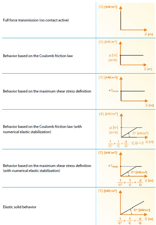 Table 2.3: Solid Contact Element
Literature
[1] Zdenek Bittnar and Jirí Šejnoha. Numerické metody mechaniky. Vydavatelství CVUT, Zikova 4, Praha 6, 1992.
[2] Ivan Nemec and Vladimír Kolár. Finite Element Analysis of Structures - Principles and Praxis. Shaker Verlag, Aachen, 2010.