Theoretische achtergrond RFEM - Berekening
1 Calculation
RFEM uses the finite element method based on the updated Lagrangian formulation and the displacement formulation.
1.1 Nonlinearity
Nature is nonlinear. Although we often look to simplify the world around us, with the increase of hardware capacity and software improvements in the last decades the linearization of real life engineering problems is not always necessary. RFEM offers a huge variety of nonlinear models covering many areas of use.
1.2 Parallelization
In order to achieve maximum computational efficiency, calculation is parallelized on different levels – the direct Cholesky linear solver is parallelized by parallel elimination of matrix rows, the dynamic relaxation method is parallelized through its natural explicit definition. Many other blocks are also parallelized (local element matrix assembly or beam cross-sectional mesh generation).
1.3 Types of Analysis
The types of deformation analysis available in RFEM can be divided into:
- Static analysis
- Dynamic analysis
- Stability analysis
1.4 Static Analysis
Nonlinearities in RFEM can be divided into the following:
- Structural nonlinearity (nonlinear releases (= hinges), nonlinear supports, etc.)
- Material nonlinearity (nonlinear elasticity, plasticity, masonry calculation, calculation of cables and membranes, etc.)
- Geometrical nonlinearity Geometrical nonlinearity is handled in RFEM according to the following user settings:
- Geometrically linear static analysis (small deformation theory, the so-called first-order theory)
- The second-order theory (P-delta analysis, improved small deformation theory taking axial forces into account)
- Large deformation theory (large deformations and large strains, nonlinear methods including the Newton-Raphson method, the Picard secant method and their combination, the so-called third-order theory)
- Post-critical analysis (large deformations and large strains, nonlinear methods including the modified Newton method and the dynamic relaxation method)
The large deformation theory and post-critical analysis differ only in the nonlinear methods used. The latter choice allows the calculation of post-critical behavior of a structure which goes through a singular point, i.e., where the stiffness matrix becomes singular. For a detailed description of the nonlinear methods, see section Nonlinear Solvers below. In case of the large deformation theory, the axial strain is computed with respect to the actual and not reference length, as in the first-order theory. Under a sufficient number of load steps, the axial strain numerically tends to a logarithmic strain definition. In case of beams computed under the large deformation theory, the axial stiffness is computed directly according to the logarithmic strain definition, which gets precise results with one load increment only.
1.4.1 Linear Solvers
The linear solvers available in RFEM are:
- Direct linear solver – parallelized Cholesky solver for symmetric sparse matrices (default choice)
- Iterative linear solver for symmetric sparse matrices
The first method is faster except for large positions, where the iterative approach can be less time demanding. The iterative linear solver, on the other hand, can be easier parallelized. The choice between the nonlinear and the linear solver is up to the user.
1.4.2 Nonlinear Solvers
Nonlinear calculations in general yield a system of nonlinear algebraic equations, which need to be solved. The robustness of the nonlinear solver is a crucial part of the calculation process within the framework of finite element analysis. The nonlinear method transforms the nonlinear problem into a sequence of linear problems, which are then solved by a linear solver. The nonlinear solvers available in RFEM are:
- Newton–Raphson method (default choice)
- Newton–Raphson combined with the Picard method Picard method (secant method)
- Newton–Raphson with constant stiffness matrix
- Modified Newton–Raphson method
- Dynamic relaxation
The Newton–Raphson nonlinear method is preferred in case of a continuous right-hand side. In case of discontinuities, the Picard method can be used (especially in combination with the Newton–Raphson as a corrector) as a more robust choice. The post-critical behavior, where the solver has to overcome limit points with singular stiffness matrices, is either solved by the modified Newton–Raphson or by the dynamic relaxation method.
1.4.2.1 Newton–Raphson
In this method, the tangential stiffness matrix is calculated as a function of the current deformation state and inverted in every iteration cycle. In the majority of cases, the method features a fast (quadratic) convergence.
1.4.2.2 Picard
This method is also known as the fixed-point iteration method. It can be thought of as a finite-difference approximation of the Newton method. The difference is considered between the current iteration cycle and the initial iteration cycle in the current load step. The method does not converge as quickly as Newton's method in general, but it can be more robust for some nonlinear problems.
1.4.2.3 Newton–Raphson Combined with Picard
The analysis starts as the Picard method and then switches to the Newton method. The idea behind this is to use the robust method far from equilibrium and the fast convergent method near equilibrium. The first n percent of iterations, for which the Picard method is used, are set in the Calculation Parameters dialog box.
1.4.2.4 Newton–Raphson with Constant Stiffness Matrix
This method is like the Newton–Raphson method. The difference is that the stiffness matrix is assembled only once in the first iteration cycle. It is then used in all subsequent cycles. Therefore, this method is faster, but not as robust as the Newton-Raphson method and the modified Newton–Raphson method.
1.4.2.5 Modified Newton–Raphson
The method is used for post-critical analysis, that is, for problems in which a region of instability has to be overcome to solve the problem. In the case of instability, where the stiffness matrix cannot be inverted, the stiffness matrix from the last stable iteration step is used. This matrix is used until the stability region is reached again. The methods enables the handling of decay diagrams:
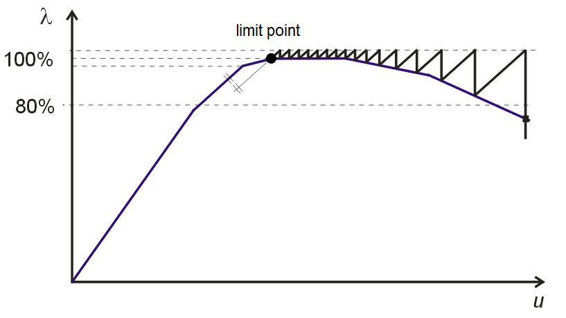
Figure 1.1: Overcoming limit point by means of the modified Newton–Raphson method
1.4.2.6 Dynamic Relaxation
This method is used for large deformation and post-critical. In this method, an artificial time parameter is introduced. Considering inertia and damping, the problem is treated as a dynamic one, using the explicit time integration method. The stiffness matrix is never inverted in this approach. The method also contains Rayleigh damping, which can be set by constants alpha, beta according to the formula:
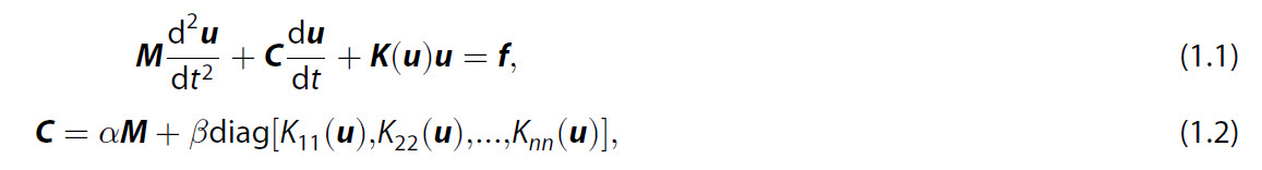
where M is the lumped (diagonal) mass matrix, C is the diagonal damping matrix, K is the stiffness matrix, dependent on the solution u in the nonlinear case, f is the vector of external forces, u is the discretized displacement and rotation vector, n is the dimension of u.
1.5 Dynamic Analysis
Dynamic calculation is available in the add-on module RF-DYNAM. Dynamic analysis contains:
- Eigenvectors
- Forced vibrations
- Equivalent loads
Forced vibrations choice can further include the following loadings
- Time history analysis
- Response spectrum method
- Multi-point response spectrum method
The response spectra method is among others used for seismic analysis. It has two possibilities:
- Linear response spectra method
- Nonlinear (push over) method
Rayleigh damping or Lehr's damping is possible to select. Rayleigh damping was described in the previous paragraph. Lehr's damping (see [1], p.264) allows the user to specify the relative damping Di of each mode independently according to equation

where omega_i is the i-th eigenfrequency, qi is the unknown solution component corresponding to the eigenfrequency omega_i, Di [−] is the relative damping corresponding to the eigenfrequency omega_i, and fi is the corresponding right-hand side.
Time history analysis is either computed by:
- Modal analysis or
- Direct integration method
The superposition rule is either square root of the sum of the squares (SRSS) or complete quadratic combination (CQC). The direct integration method is based on the implicit Newmark method, which is second order accurate in time and absolutely stable. The Newmark method uses a constant time step approach.
The following types of mass matrix definition are available
- Diagonal (lumped) mass matrix
- Diagonal (lumped) mass matrix with rotational elements (improved version)
- Unit mass matrix
1.6 Stability Analysis
The stability calculation is available in the add-on module RF-STABILITY. Two methods for stability calculation are available:
- Linear eigenvalue analysis
- Nonlinear stability analysis (nonlinear calculation, load is increased until structure failure, the critical load factor is determined)
For the linear eigenvalue analysis four methods are available:
- Lanczos method
- Calculation of the roots of the characteristic polynomial
- Subspace iteration method
- Improved Conjugate Gradient (ICG) iteration method
1.7 Member Calculation
In RFEM the following types of members can be computed:
- Beam (Bending resisting member that can transmit all internal forces)
- Rigid member (Coupling member with rigid stiffness. It is internally modelled by a high stiffness value, which is set automatically by a couple of orders higher than the surrounding construction, which allows the member to behave rigidly and to be numerically stable at the same time.)
- Rib (Downstand beam considering the effective slab width)
- Truss (Beam with moment releases at both ends)
- Truss (only N) (Member with stiffness EA only)
- Tension (Truss (only N) with failure in case of compression force)
- Compression (Truss (only N) with failure in case of tensile force)
- Buckling (Truss (only N) with failure in case of compression force > Ncr)
- Cable (in compression it loses its stiffness, has to be calculated with the large deformation option only)
- Cable on pulleys (Member on polyline, can only be shifted in longitudinal direction, absorbing tensile forces only (pulley))
- Definable stiffness (Member with user-defined stiffnesses, without necessity to define cross-section)
- Coupling rigid–rigid (Rigid coupling with bending resisting connections at both ends)
- Coupling rigid–hinge (Rigid coupling with bending resisting connection at member start and hinged connection at member end)
- Coupling hinge–rigid (Rigid coupling with hinged connection at member start and bending resisting connection at member end)
- Coupling hinge–hinge (Rigid coupling with hinged connections at both ends – only axial force is transmitted
- Spring (Member with spring stiffness, incl. nonlinear behavior)
- Dashpot (Parallel combination of viscous dashpot and elastic spring i.e. Kelvin–Voigt model. In static analyses, only the spring part is taken into account.)
A large database of cross-sections is available in RFEM. Hybrid beams, which allow more than one material for the cross-section, are also supported. Each beam can be further equipped by a release (= hinge, in general nonlinear) on each side.
1.8 Plate and Shell Calculation
Two types of plate theories, with respect to the transversal shear approximation, can be selected:
- Mindlin theory (linear shear theory, default choice)
- Kirchhoff theory (no transversal shear considered, suitable only for thin plates). The Kirchhoff theory is available only for linear calculations.
The types of surfaces / plates in RFEM:
- Surfaces with material orthotropy – plates of constant thickness with orthotropic material defined by six elastic constants
- Surfaces with geometrical orthotropy – surface with periodically varying thickness. By the so-called smeared stiffness approach, the 8×8 average stiffness matrix is assembled. The list of all plates of these types, supported in RFEM, follows:
- Effective thickness (orthotropic material possibility)
- Defined by stiffness matrix (This plate type allows the user to define an arbitrary plate defined by an 8×8 stiffness matrix. This definition allows the definition of unsymmetric compositions also. Initial calculation of the stiffness matrix can be made outsideand imported into RFEM easily from Excel (and exported also)).
- Coupling
- Unidirectional ribbed plate
- Bidirectional ribbed plate
- Trapezoidal sheet
- Hollow core slab
- Grillage
- Unidirectional box floor
- Without tension surface – plate made of isotropic material. The calculation is nonlinear due to the effect occurring, for example, in masonry walls: under tension the plate loses its in-plane stiffness. Bending is handled linearly.
- Rigid plate – plate with rigid stiffness. It is internally modelled by a high stiffness value, which is set automatically by a couple of orders higher than the surrounding construction, which allows the plate to behave rigidly and to be numerically stable at the same time.
- Laminated plate – RFEM allows the analysis of laminated plates (= multilayered plates). Any number of layers with material orthotropy is allowed. An unsymmetric composition is supported. The transversal shear calculation is based on the Grashoff formula. Stress/strain dependence throughout the plate thickness can be shown graphically in any point of the plate.
- Safety glass – safety (laminated) glass is a multilayered plate consisting of glass and foil layers. The elastic properties of glass and foil differ significantly – by a couple of orders. Due to the significant difference in stiffness, there is a significant difference in the angles of the normal lines (the deformed points are connected to create the normal lines in each layer). These special plates are solved by solid elements to handle the situation accurately.
- Insulating glass units – in insulating glass units, glass layers (or safety glass layers) are combined with gas layers. Gas is simulated by solid elements (see the section List of All Elements for more details). Large-deformation calculation is necessary in this case. The calculation allows the consideration of solar flux radiation and infinite ray reflections in the glass unit.
- Membranes – surfaces with no bending stiffness (textile, for example). Isotropic as well as orthotropic membranes can be defined. The calculation is nonlinear due to the effect which occurs in real membranes – under compression the membrane loses its stiffness. Membranes can be calculated only with the large deformations. Let us note that RFEM also has the feature of nonlinear form-finding techniques, which allows finding the unknown shape of a membrane surface that is useful in membrane structure design (circus tent design, for example).
Note, that curved surfaces in RFEM are approximated by planar finite elements. In nodes where planar elements are joined, deformations and rotations are forced to be equal. This approximation converges with a finer mesh to exact values on curved surfaces.
1.9 Load
Loads in RFEM can be defined in many different ways:
- Nodal load (force load, moment load, imposed deflection load, imposed rotation load)
- Line Load (force intesity load, moment intesity load, imposed deflection load, load can vary along the line length)
- Member Load (force intesity loading, moment density loading, temperature loading, axial strain loading, axial displacement loading, precamber loading, initial/end prestress loading, displacement loading, rotation loading, pipe loading, rotary motion loading, imperfection loading, loading can vary along the member length)
- Surface Load (pressure loading, temperature loading, strain loading, precamber loading, rotary motion loading)
- Solid Load (force intesity loading, temperature loading, strain loading, buoyancy loading, rotary motion loading)
- Free concentrated load – A free concentrated load acts as a force or moment on any location of the surface.
- Free Line Loads – A free line load acts as a uniform or linearly variable force along a freely definable line of a surface.
- Free rectangular / circular / polygon load – A free rectangular / circular / polygon load acts as a uniform or linearly variable surface load on a rectangular / circular / polygon, freely definable part of a surface.
1.10 Support
RFEM features the following kind of supports:
- Nodal support
- Line support
- Surface support (implementation is based on the subsoil implementation described in the next point)
- Subsoil simulation (using two models – Winkler subsoil and Pasternak subsoil, which allows the definition of shear stiffnesses in the subsoil)
Nodal and line supports can act with respect to any degree of freedom (ux, uy, uz, fix, fiy, fiz), can work in the rotated coordinate system, and it is possible to add linear springs in any direction.
Nodal supports are further equipped with many nonlinearities like nonlinear springs defined by a multilinear diagram, by partial activity behavior (not acting in the case of positive or negative force in a particular direction), or by friction (stiffness dependence on force in a particular direction). Linear and surface supports are further equipped by partial activity behavior (not acting in case of positive or negative force in a particular direction).
1.11 Release
Two types of releases are available in RFEM:
- Nodal release
- Line release
A release (= hinge) between two nodes allows the connection of any degree of freedom (ux, uy, uz, fix, fiy, fiz), allows the definition of linear stiffness between any degree of freedom, and is also equipped with nonlinearities: nonlinear hinge behavior defined by a multilinear diagram, partial activity behavior and fixed-under-condition behavior (fixed, if My is positive, for example). A special possibility is a scissor release. With a scissor release, you can model crossing beams. For example, there are four members connected at one node. Each of the two member pairs transfers moments in its continuous direction, but they do not transfer any moments to the other pair. Only axial and shear forces are transferred in the node. A line release in RFEM allows linear behaviour only.
1.12 Material Models
RFEM contains an extensive database of materials from various technical standards and company specifications (steel, concrete, glass, foils, wood). Special materials available in RFEM are gasses (in RFEM solved using solid elements, see the description of finite elements used in RFEM below) and materials with temperature dependent properties. From the modelling point of view, all materials can be modelled using different material models:
Linear material models:
- Isotropic Linear Elastic
- Isotropic Thermal-Elastic (elastic parameters are temperature dependent)
- Orthotropic 2D (calculations of wood, carbon fiber materials etc.)
- Orthotropic 3D (calculations of wood, carbon fiber materials etc.)
Nonlinear material models:
- Isotropic Plastic 1D (fully plastic model with plastic strains, arbitrary cross-sections)
- Isotropic Plastic 2D/3D (fully plastic model with plastic strains, the von Mises hypothesis)
- Nonlinear Elastic 1D (nonlinear calculation without considering plastic strains)
- Nonlinear Elastic 2D/3D (nonlinear calculation without considering plastic strains, according to the following hypotheses: von Mises, Tresca, Drucker–Prager, Mohr–Coulomb)
- Orthotropic Plastic 2D (plastic calculations of wood, based on the Tsai–Wu hypothesis)
- Orthotropic Plastic 3D (plastic calculations of wood, based on the Tsai–Wu hypothesis)
- Isotropic Masonry 2D (calculation of masonry walls using maximum tensile limit stresses)
In practice it is often necessary to model materials which have different yield limits in tension and in compression. The material models which can handle these effects are the following:
- Nonlinear Elastic 1D
- Nonlinear Elastic 2D/3D (only the Drucker–Prager and Mohr–Coulomb hypotheses)
- Orthotropic Plastic 2D
- Orthotropic Plastic 3D
Isotropic hardening is implemented in all of the above mentioned material models. The latter three models (Orthotropic Plastic 2D, Orthotropic Plastic 3D and Isotropic Masonry 2D) allow the definition of bilinear hardening, all other nonlinear material models allow the definition of multilinear hardening, defined by a diagram). Kinematic hardening is not available. Another feature is the calculation of cables (special type of member) and membranes (special type of surface), which have no bending and compression stiffness. The calculation process lowers the stiffness in compression, which makes the calculation nonlinear. Large deflection theory (third order theory) is necessary to be used in that case.
1.13 Construction Models
The following construction models can be selected:
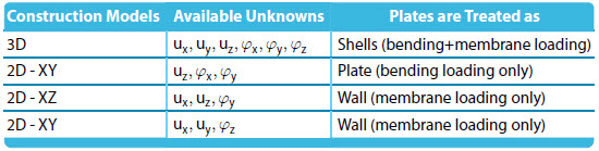
Table 1.1: Construction Models in RFEM
1.14 Appendix - Second Order Analysis
Second-order analysis is on the half way between the first-order theory (small deformation theory) and the large deformation analysis. The small deformation theory is calculated in the undeformed configuration, the resulting equations are linear and therefore no iterations are needed. The large deformation analysis, on the other hand, is calculated in the deformed configuration, which is updated in each iteration. The resulting equations are therefore nonlinear. As part of the large deformation theory, the effect of axial forces on the bending stiffness is considered (the so-called P-delta/P-Delta effect). Tensile forces increase the bending stiffness, compressive forces decrease the bending stiffness. The second-order analysis is calculated in the undeformed configuration, however, the effect of axial forces on the bending stiffness is considered. If axial forces are supposed to be known, then the problem is linear and can be therefore solved within one iteration. If axial forces are unknown, which is the usual case, the problem is solved iteratively as a sequence of linear problems, in which the axial force is updated from the previous iteration and considered constant within the particular iteration step. This numerical approach is in fact the fixed-point iteration method, in RFEM called equivalently the Picard method. The Newton method is not available for this type of analysis [1]. Let us clarify the second-order analysis on the beam equation (see Petersen, Statik und Stabilität der Baukonstruktionen, 1982, p.187)
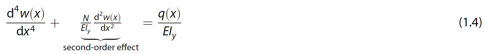
where w(x) is the beam transversal deflection, N is the axial force (N > 0 means tensional force), E is Young's modulus, Iy is the bending moment of inertia and q(x) is the pressure load. We easily see that by considering the axial force N constant, the equation is linear. If the axial force N is zero, then the equation (1.4) reduces to the standard Euler–Bernoulli beam equation. In RFEM the second-order theory is available not only for beams, but also for plates and solids.
[1] The Newton method could be used in general. This would require to express the axial force N in terms of unknown deflections
and rotations, the resulting equations would be nonlinear. However, this approach is not used in RFEM.